Search and information retrieval
In the previous blog post we looked at why and how we always have to transform and preprocess the court and authority decisions we download, to make our data suitable and ready for legal work.
We have finally reached one of the most obvious uses for legal practitioners: legal search, and its pitfalls. Let us see what search means for us and what methods are available.
‘grep’ and manual search
The oldest machine method is to open a text file, read it into the computer’s memory, then send the memory cells one after the other to the central processing unit, which compares the value read with the value searched for. We still do this the same way as in the fifties, only much faster. Reading, memory and the CPU are all so fast that in most cases we need no other method: no dedicated database, no index. The catch is that, thanks to the “progress” of operating systems and user interfaces, most users no longer really have access to this simple method, may not even know about it, or the operating system (e.g. Windows or Android) does not offer a built-in solution optimised for this approach.
This is why it is worth getting to know the program (or family of programs) called “grep”, which gives us a realistic picture of the “ancient”, raw power of search today. Unfortunately, it is not part of a default Windows installation, but it is part of Linux distributions and macOS. If you want to search the Collection of Court Decisions (BHGY) in this raw, text-based form, I strongly recommend trying it, e.g. the free ripgrep. On Windows, the command line offers the FIND command inherited from DOS (do not use it, it is not worth it), the “findstr” command, also available for twenty years now and working much like grep, or, in PowerShell, the “Select-String” command.
Suppose we want to search the whole BHGY (225,407 files in 2,907 folders, 6.5 GB of text). Let us search the BHGY for a word that occurs often (in this case “elektronikus”, meaning “electronic”, 37,196 hits) and for an exact two-word phrase that rarely gives a hit (in this case my own name, only five hits):1
| tool | search: “elektronikus” | search: “Homoki Péter” |
|---|---|---|
| ripgrep -F | 8.8 seconds | 14 s |
| GNU grep 3.0 | 28 s | 63 s |
| findstr /s /m /l | 21 s | 23 s |
| find.exe | 537 s | 693 s |
| PowerShell Select-String | 287 s | 301 s |
It is no accident that agentic frameworks also use grep for search by default: in many cases there is no need to build indexes or set up any more complex search workflow. From the search instruction, the large language model works out which keywords to search for with grep, then collects the results and filters them further if needed.
In professional use, however, this method also has many drawbacks that should not be forgotten: if we get too many hits, or if we search for one word form but also want hits for other, similar words (e.g. when searching for “szerződés”, contract, also for “megállapodás”, agreement).
Indexing
Indexing is an ancient method that also works on paper and helps to speed up searches. The same can be done electronically, and on desktop operating systems (that is, not on phones and tablets) it is now a basic feature: Windows Search on Windows, Spotlight on macOS, and on Linux an application that depends on the distribution (e.g. LocalSearch, Baloo). On Windows, make sure under Settings that the content you want to search is actually indexed, which depends on where it is stored (see “Privacy & security”, “Search”, “Find my files”: with the Classic setting, the content to be indexed must be within the listed locations, e.g. inside Documents, or you have to add the folder manually).
These indexers work like this: when first started, the operating system builds itself a directory structure, walks through it to collect the individual files, and, according to their type (format), extracts the features used for searching, including the content of text files (and for music files, e.g. the artists and album names). When a new file is created (or copied), the indexer is notified about it so that it will examine and index it in due course. Depending on how sophisticated the program is, it often applies the preprocessing steps we met in the previous post (splitting into words, stemming, normalisation, filtering out the most frequent words such as articles). The actual search naturally works from an inverted index, because for a fast search we want to know which files contain a given word (and not which words a given file contains).
But if we try Windows Search on the BHGY folder (if it is an indexed folder), chances are that after 30 minutes of searching we will not get a single hit. Of course the index could be rebuilt, and the real cause of the error could surely be tracked down in every case, but frankly, the built-in indexes of operating systems do not always work reliably enough. For professional work, therefore, dedicated applications are often used, with indexes they build and store in separate databases, because their operation is not affected by the possible malfunction of a hundred other processes.
In our case, for example, the SQLite database engine built the 4 GB index of the BHGY in 959 seconds, after which we got the following values:2
| tool | search: “elektronikus” | search: “Homoki Péter” |
|---|---|---|
| SQLite FTS5 | 0.011 seconds | 0.0001 seconds |
SQLite is therefore about a thousand times faster than ripgrep for the one-word search, and about a hundred thousand times faster for the two-word phrase.
Searching Hungarian-language decisions in ordinary legal work never needs such speed. So when does indexing make sense, when is it worth the time and energy?
On the one hand, when we want to search the dataset very often, for example when the index is used not by one person but by several users.
On the other hand, when we want to see as hits not only the exact word or phrase but also its forms with other suffixes: for example, a search for “tó” (lake) should also find “tavat” (lake, in the accusative), “Törvényszék” (regional court) should find “Törvényszékkel” (with the regional court), “szuverén” (sovereign) should find “szuverenista” (sovereigntist), and “húsz” (twenty) should find “20”, “huszat” and “huszad”. This is not a trivial task, because nobody is happy to get hits they consider unjustified: such “false positive” hits make searching just as hard. For example, a search for “lehet” (may, can) should not return every form of the verb “to be” (e.g. “van”, is), and a search for “vádlott” (the accused; 4,714,322 hits) should not return “vádli” (calf of the leg; another 164 hits).
If in such cases we want more than exact hits, one option is to insert an intelligent step before the raw (e.g. grep) search, that is, to list every possible word form one by one (or let the search agent do it for us, because it recognises that this is needed). The other option is to use an index and apply stemming or lemmatisation when building it, as the words are collected. Stemming is the simpler and faster solution, but depending on the stemmer used, it can produce many false positive hits.
One of the most effective solutions is “Hunspell”, developed by László Németh.3 This excellent Hungarian-developed spell checker is used, for example, by LibreOffice and Firefox (and not only for Hungarian); its large dictionary and rule set also make it suitable for stemming. It is not flawless at stemming, though: it struggles with the “van”–”lehet” problem mentioned above, and it gives “perbelibeli” as the stem of “perbeli” (in the lawsuit). Lemmatisation is far more resource-intensive; one example is huspaCy,4 published by György Orosz, the Hungarian model of the popular spaCy,5 a free neural network library for language processing. But we find that huspaCy is not flawless on our corpus either: for “Ítélőtáblához” (to the Regional Court of Appeal) the lemma becomes “Ítélőtáblá”. Hunspell’s errors mainly affect verbs and huspaCy’s mainly proper names, so the obvious idea is that the fastest solution is to run Hunspell’s suggestions over huspaCy’s output and record Hunspell’s version where they differ.
Here is an (estimated) cost-benefit comparison of the solutions in a table (measured on my own configuration, with a small GPU):
| method | error rate | processing time |
|---|---|---|
| Hunspell | 3.3% | 35 minutes |
| huspaCy | 0.8% | 20.5 hours |
| Hunspell+huspaCy | 0.4% | 21 hours |
Ranking the hits (reranking) and BM-25
Sometimes there are too many hits to read them all. And even if we can read them all, we get them back in the order of the raw source text or of the index build, which is very rarely what we want. So it helps to have a better method for ordering and displaying the hits.
For the BHGY, ordering can be helped by grouping the hits, for example, by court level or by year of decision, so that later hits from the Curia (the Supreme Court of Hungary) come before earlier Curia hits or hits from district courts. These are professional orderings that can be set by hand and are tied to the nature of the specific corpus.
There are also general methods built on linguistic and statistical grounds, independent of the specific dataset. Briefly, for learning’s sake, let us look at the basics of one of the most popular methods (BM-25). If the searched word occurs several times in a decision, that decision ranks higher among the hits (“term frequency” or “TF”). On its own, the drawback of this is that for frequent words longer documents will always rank higher, so instead of comparing how many times the word occurs (e.g. 5 times), the methods often compare its share of the document’s total word count (e.g. 0.0005) and rank the hits by that. The method has another element, however, which in multi-word searches tries to make the rarer, but often more important, word carry more weight among the hits. Take the case where we want to find hits about the electronic signature used by the plaintiff, and we are not interested in an exact phrase (e.g. we are not searching for the phrase “felperesi elektronikus aláírás”, the plaintiff’s electronic signature), but each word must appear exactly. The word “felperes” (plaintiff) appears in 80% of BHGY decisions, “elektronikus” (electronic) in 16%, and “aláírás” (signature) in only 4%; any of the three words appears in about 84% of decisions, and all three in 1%. If we look at the 84% list (any of the three words), the first fifty hits will be dominated by decisions in which the generally most frequent word, “felperes”, appears most often. The best hit will be the one in which the most frequent of the three words, “felperes”, appears disproportionately often relative to the length of the decision. Neither “elektronikus” nor “aláírás” will appear even once in the first fifty hits. If we bring in the measure of “inverse document frequency” (“IDF”), rarer words will carry more weight among the hits. In our example, the IDF of “felperes” will be 0.22 and that of “aláírás” 3.14, and thanks to this the best hit will be the decision in which “elektronikus” appears 44 times and “aláírás” seven times. Based on these two elements this ranking method is called TF-IDF, because the score that decides the order is the product of the two measures. BM-25, the most widely used method today, refines this relatively simple method in two respects (correcting certain distortions caused by “too frequent” words within one text and by disproportionately long texts).
Let us admit that this kind of ranking methodology is hard for the typical legal practitioner to stomach. It would be hard to weigh, before each search, what the right search strategy would be for the legal problem at hand, and with what parameters we would like to get the best hits, e.g. what the optimal k1 and b values of BM-25 should be. So we ignore the details and blindly trust the algorithm and the settings of the search engine’s developer. This is also why the typical search strategy is usually to narrow down too many hits with one or two more words or with a legally meaningful filter, such as the deciding court or the date of the decision.
Dense and sparse text embeddings and their use in search
In ranking we saw the statistical method in which words and documents are turned into some kind of “numbers”, and the best hit is decided on that basis. This mathematical approach is also expressed by saying that each document is in fact a high-dimensional vector, in which each dimension gives the frequency of one of all the possible words (in the given index or corpus). Besides the document vector, the query is also treated as such a vector, so the BM25 value will be the dot product of the query vector and the document vector. Projecting a text onto such a vector is called embedding.
This kind of embedding, also used in BM-25, is called sparse embedding, because there are many words, the number of dimensions is large, and most dimensions of the vector are zero (the words that do not occur in the document). Each dimension is one word, every dimension can be read (how frequent the given word is), and the dimensions are not related to each other. It is a very fast method built on computed vectors, because no long and costly machine learning process is needed to get the result.
However, it is not a good method for taking into account related words, synonyms or, in general, relations of meaning, such as that “terhelt” (the defendant) in a decision can mean either an accused (“vádlott”) or a suspect (“gyanúsított”). So if we search for “szerződés” (contract), even with lemmatisation we will not get a decision that only uses the word “megállapodás” (agreement), and if we search for “elektronikus” (electronic), we will not get the decisions containing the word “digitális” (digital).
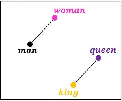
There are methods that try to take this into account as well. One of the most obvious is the use of “dense embeddings”. For the sparse embedding of the BHGY, we worked with 1 million and 2 million dimensions respectively when turning the text into vectors (1 million with lemmatisation, 2 million without); the zeros are not stored, and of all the 1 million dimensions, only 0.079% hold any value. Dense embeddings are called dense because every dimension holds a value; this is why (depending on the specific recipe) they use only a few hundred or at most a few thousand dimensions. But these numbers do not refer to specific words or concepts and have no meaning a human could interpret; each is really just a coordinate used to evaluate the meaning of texts.
Such a dense embedding can only be created through a machine learning process. It is not realistic for us to start such training from scratch, because it would take a great deal of time and money: only with text at least a hundred times larger than the BHGY corpus would we stand a chance of starting a pre-training that could even approach the capabilities of the leading embedding models. This phase can even be the same as the similar pre-training phase of typical large language models (the best embedding models, e.g. Gemini Embedding and Qwen Embedding, indicate precisely that this phase was shared with the models used for “chat”). After that, however, we will need a few tens of millions of simpler question–answer style text pairs, which show which texts are close to each other in real texts.
Since we use the embedding model for information retrieval here, it makes sense to fine-tune it at the end for the specific information retrieval task as well: that is, to teach it what answers lawyers typically expect to which questions, which answers we are happy with.
In practice this means that we do not train such an embedding model ourselves, but simply download the end result that someone else has trained. Ultimately, we hope that for our task, searching Hungarian court decisions, it will be a near-optimal solution.
In concrete terms, a dense embedding model is used like this: we split the text we want to search, the cleaned BHGY dataset, in the way the chosen model expects, and turn the text chunks into vectors, that is, we “embed” the text into an easily searchable vector form. When searching, we embed the query with the same model and look for the vector of the transformed BHGY text that is closest to the query vector. We find it by taking the dot product of the query vector with every stored vector (for normalised vectors this is the cosine similarity) and selecting the largest products at the end (e.g. the 50 best hits). The best hit is the text chunk with the largest product. From the best hits we look up the original text chunks that belong to the best vectors. Since the BHGY contains a great many decisions, we store the vectors in a fast vector database (with a vector index) for the speed we need.
As we will see below, the drawback of the method is that the text chunks are relatively small, e.g. typically 512 word pieces (tokens), which means less than a page of text per chunk. This solution will not yet see deeper legal connections or draw legal conclusions for us. In other words, it will not be able to put the kind of deep legal intelligence behind the search operations that we would often need. For that we will need other methods requiring much more thought and experimentation, e.g. richer semantic information, deeper analysis and semantic enrichment of court texts, legal ontologies and argumentation modelling, and LLM agents that use them.
Evaluation
Before concluding, let us briefly look at how we can decide which of the many downloadable embedding models to use for this task. Here, too, we have to return to the operation of evaluation, mentioned several times before.
One option is to rely on evaluations run by others, for example on one of the leaderboards published on Hugging Face, the one that compares the performance of embedding models (MTEB: Massive Text Embedding Benchmark).6 But which one? No leaderboard specifically for Hungarian has been published, but there is one for English, one called European (with 28 languages) and a general multilingual one. We can also filter the tables, e.g. to see the results of each model in the legal domain. In our case we are of course interested only in models that work with text, but we also have to decide which evaluation method’s results interest us: the European table alone publishes results on 73 different tasks, which we can average. There are, for example, two hundred German legal questions in German,7 or the classification of Greek legislation, and so on. It is not easy to decide which evaluation really fits the search needs of a Hungarian lawyer, just as the average over 73 tasks is not necessarily informative either.
For the sake of the experiment, I put together two separate evaluation sets. For the first, I wrote down 14 Hungarian legal questions that I consider difficult, plus a larger collection of statutes and legal literature from which they can very probably be answered (and hopefully in the same way). The evaluation was whether, for each question, the model ranks the best source material of the collection first. My aim was that these should be questions arising in a lawyer’s work that a practising lawyer would answer, e.g. question: “in a licence agreement for a copyright work to be created in the future, can the warranty claims under the Civil Code (Ptk.) be enforced in the absence of an express provision?”; answer: “no, because under the Copyright Act the rules of the Civil Code apply only secondarily, that is, in matters the Copyright Act does not regulate, while the Copyright Act lays down a specific procedure for correcting works to be created in the future” (my translation). Then, based on the hand-written examples and the legal literature, I had a large language model generate further questions of similar complexity (another 243). (For copyright reasons, I unfortunately cannot share the evaluation texts and examples.)
In the other test set, the task was to find the BHGY decision belonging to a summary published by the National Office for the Judiciary (OBH) for the BHGY (and produced by machine learning models). For example, for “No conclusion can be drawn, in itself, from possibly unlawful findings of fact or from a possible failure to give reasons, in the absence of an indication of the substantive legal provision, as to why the courts that acted in the case acted unlawfully. Act III of 1952, Section 206(1)” (my translation), the answer is judgment Mfv.10165/2019/7. This set also has 500 questions. Here the search did not run on the whole BHGY but on 5,000 decisions (the 500 correct decisions plus further randomly selected ones), and I used only the first 4,000 characters of each decision.
The measure of the comparison below is the so-called “hit” value: for what percentage of the questions the correct answer was in first place, in the top three, or in the top ten. “Method” shows which models or ranking method I used (except for BM25, all are dense embedding models). There is also a hybrid method (e.g. BM25+Gemini), in which we rank the hits both with the traditional (non-machine-learning, sparse embedding) method and with the dense, semantic embedding models, then the two hit lists are merged and the final score is given on that basis. The other novelty is reranking, in which the results of the hybrid solution are not merged mechanically but with the help of another, specially trained model (in this case bge-reranker-v2-m3). Its task is to score the given question–answer pairs, that is, how well the given answer fits the given question, and on that basis to rescore the top twenty. As we can see, this greatly improved the scores on the question–answer task, typically with short questions, but it worsened the scores on the BHGY summaries, because the question–decision pairs had to be cut to 512 tokens, so it saw only the beginning of the long decisions.
257 questions
| Method | hit@1 | hit@3 | hit@10 |
|---|---|---|---|
| BM25 plain | 38.5% | 59.9% | 73.2% |
| BM25 lemmatised | 49.8% | 73.2% | 85.6% |
| bge-m3 | 49.8% | 73.2% | 87.5% |
| snowflake-arctic-embed-l-v2 | 60.3% | 79.4% | 91.4% |
| Qwen3-Embedding-8B | 47.5% | 75.5% | 90.3% |
| OpenAI large | 46.7% | 68.1% | 81.7% |
| Gemini | 54.5% | 82.5% | 94.6% |
| BM25 lemmatised + Gemini | 57.2% | 82.9% | 94.6% |
| + reranking (top 20) | 76.3% | 92.6% | 96.9% |
Finding the decision from its BHGY summary
| Method | hit@1 | hit@3 | hit@10 |
|---|---|---|---|
| BM25 plain | 18.2% | 27.4% | 36.8% |
| BM25 lemmatised | 21.2% | 31.2% | 42.2% |
| bge-m3 (1024 tokens) | 9.2% | 15.4% | 26.0% |
| snowflake (1024 tokens) | 12.2% | 19.4% | 30.2% |
| Qwen3-8B (1024 tokens) | 12.2% | 22.6% | 34.2% |
| OpenAI large | 15.0% | 24.8% | 34.8% |
| Gemini | 24.8% | 34.8% | 48.0% |
| BM25 lemmatised + Gemini | 26.0% | 37.0% | 48.4% |
| + reranking (top 20) | 12.2% | 21.0% | 38.8% |
I also examined a few other models (Jina v3, E5, EmbeddingGemma, huBERT, OpenAI small), but they did not give better results than the ones above, so the tables show only the typical models. (Jina v3 was the best open model on the BHGY task, with a hit@10 of 41.0%.) Looking at the results, we can see that in searching BHGY summaries only Gemini did better than lemmatised BM25. For the 257 questions, using the two methods (sparse and dense embedding) together brought a significant improvement over lemmatised BM25.
Summary
I hope I have managed to show the power of raw search and the advantages of indexing, ranking and semantic embeddings: when they are useful and when not to count on them. This brings us to the end of the foundational part of the series, and I ask for a few weeks’ patience before it continues, because with the end of the year approaching, every free minute has to go to tasks that are urgent for others.
The values show the smallest of three searches, except for find and Select-String, where we only had the patience for one run. As find.exe is an ancient relic, you have to tell it by hand which files to search, so we do not recommend it for this purpose at all. ↩
These values refer to the second run, when the whole index had already been read into the computer’s memory. ↩

